Mental Health Analysis - Kaggle Competition

Mental health is a critical aspect of well-being, influencing daily life, work productivity, and overall quality of life. In recent years, the prevalence of depression has surged, making it imperative to identify trends and underlying risk factors early.

This project, developed as part of a Kaggle competition, aims to build a machine learning model capable of predicting depression based on various social, psychological, and demographic indicators. By analyzing these features, we hope to provide insights that can be used for early intervention and better mental health support.

Exploratory Data Analysis (EDA) plays a critical role in understanding the dataset, identifying trends, and ensuring data quality before modeling. Through this process, we identified several important insights that shaped our data preprocessing strategy.

One of the first challenges encountered was missing data. Six key features contained significant amounts of missing values, which needed careful handling (Table 1 and 2). Since missing values can lead to biased predictions and unreliable models, we assessed different imputation techniques and removal strategies. The decision on whether to impute or remove missing values depended on the proportion of missing data and the relevance of the affected features to our predictive goal.

# Table 1: Feature Overview: Non-Null Counts & Data Types 

+----+---------------------------------------+---------------------+-----------+
|    |             Column Names              | Non-null values (%) | Data Type |
+----+---------------------------------------+---------------------+-----------+
| 0  |                  id                   |        100.0        |   int64   |
| 1  |                 Name                  |        100.0        |  object   |
| 2  |                Gender                 |        100.0        |  object   |
| 3  |                  Age                  |        100.0        |  float64  |
| 4  |                 City                  |        100.0        |  object   |
| 5  |    Working Professional or Student    |        100.0        |  object   |
| 6  |              Profession               |       73.966        |  object   |
| 7  |           Academic Pressure           |       19.827        |  float64  |
| 8  |             Work Pressure             |       80.158        |  float64  |
| 9  |                 CGPA                  |       19.828        |  float64  |
| 10 |          Study Satisfaction           |       19.827        |  float64  |
| 11 |           Job Satisfaction            |       80.163        |  float64  |
| 12 |            Sleep Duration             |        100.0        |  object   |
| 13 |            Dietary Habits             |       99.997        |  object   |
| 14 |                Degree                 |       99.999        |  object   |
| 15 | Have you ever had suicidal thoughts ? |        100.0        |  object   |
| 16 |           Work/Study Hours            |        100.0        |  float64  |
| 17 |           Financial Stress            |       99.997        |  float64  |
| 18 |   Family History of Mental Illness    |        100.0        |  object   |
| 19 |              Depression               |        100.0        |   int64   |
+----+---------------------------------------+---------------------+-----------+
                    

Another major finding was the severe class imbalance in the target variable, Depression. Less than 20% of individuals in the dataset were labeled as depressed, indicating a strong skew towards the non-depressed class (Figure 1). This imbalance can lead to models that are biased towards predicting the majority class, reducing their ability to detect cases of depression accurately. To address this, we considered resampling techniques such as Synthetic Minority Over-sampling Technique (SMOTE) and undersampling. Additionally, evaluation metrics such as F1-score and/or Recall were prioritized over accuracy to ensure the model's performance remained fair across both classes.

# Figure 1: Distribution of the target Label (Depression)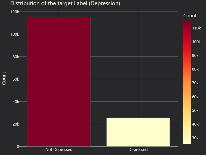

We also examined feature correlations with depression. While some features, such as Gender and Family History of Mental Illness, showed little to no correlation with depression, others displayed strong associations (Figure 2 and 3). Suicidal Thoughts emerged as the most predictive factor, followed by Academic Pressure, which suggested that high stress levels in education contribute significantly to mental health struggles (Figure 4 and 5). Age was also a key factor, with certain age groups appearing more vulnerable to depression. Furthermore, Occupation played a role, with noticeable differences in depression prevalence between students and professionals (Figure 6 and 7). These insights guided our feature selection process, allowing us to focus on variables with the most predictive power.

# Figure 2: Gender vs. Depression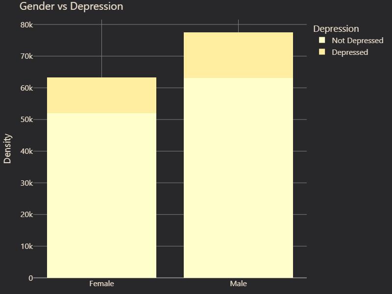

# Figure 3: Mental Illness vs. Depression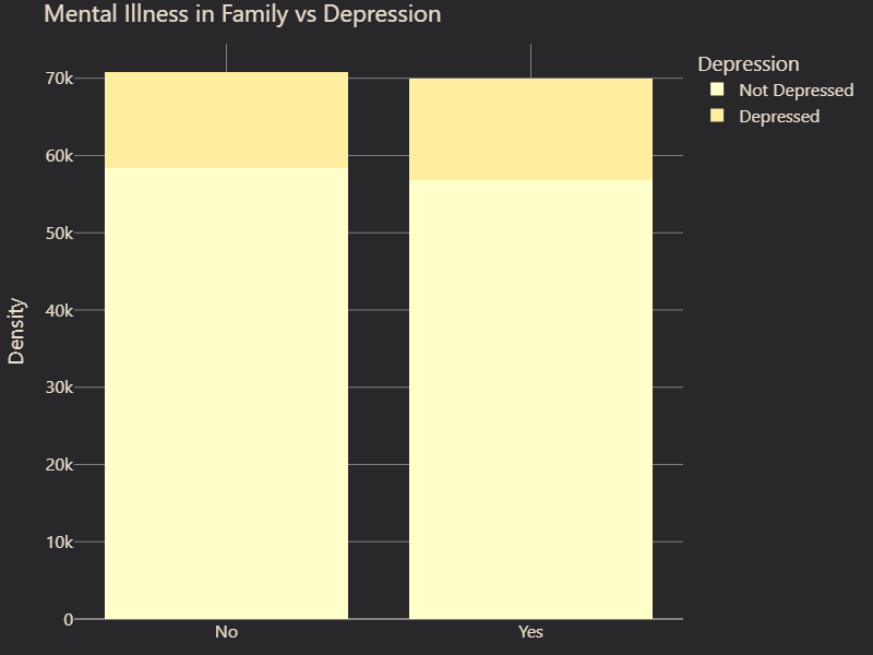

# Figure 4: Suicidal thoughts vs. Depression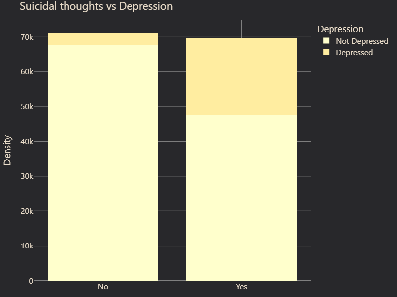

# Figure 5: Academic pressure vs. Depression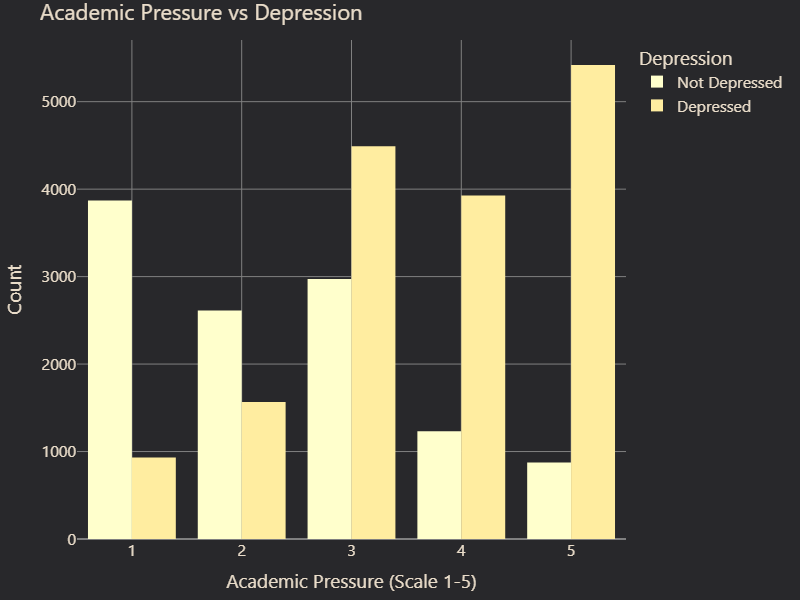

# Figure 6: Work pressure vs. Depression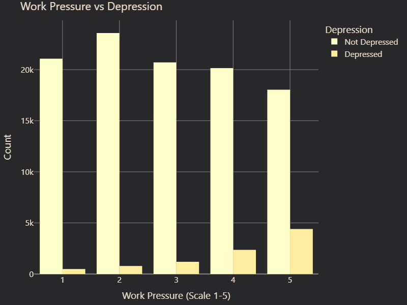

# Figure 7: Occupation vs. Depression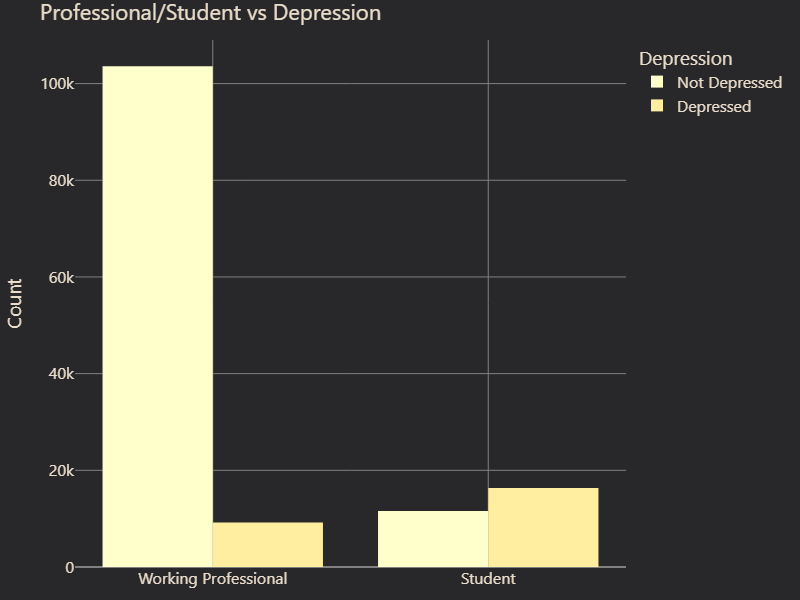

Moving forward, these findings provided a clear roadmap for preprocessing. The next steps involved handling missing values, implementing techniques to mitigate the target imbalance, and selecting the most relevant features for modeling. By taking these steps, we ensured a robust foundation for predicting depression, improving both model reliability and interpretability.

Feature engineering and data cleaning are critical steps in the machine learning pipeline, ensuring that the dataset is refined, structured, and optimized for model performance. Without proper feature selection and preprocessing, a model can be misled by noisy or irrelevant data, ultimately leading to inaccurate predictions.

Handling Missing and Irrelevant Features

Several features in the dataset, such as Profession, Name, and id, were found to be poorly correlated with the target label. While these features may carry some contextual information, they do not contribute meaningfully to predicting depression and therefore were removed to reduce noise and enhance model efficiency. Additionally, features such as CGPA were only applicable to students, limiting its generalizability for working professionals in the dataset. Due to these limitations, these features were dropped.

# Table 2: Feature Overview: Null Value Counts  

+----+---------------------------------------+-----------------+-----------+
|    |             Column Names              | Null values (%) | Data Type |
+----+---------------------------------------+-----------------+-----------+
| 0  |                  id                   |       0.0       |   int64   |
| 1  |                 Name                  |       0.0       |  object   |
| 2  |                Gender                 |       0.0       |  object   |
| 3  |                  Age                  |       0.0       |  float64  |
| 4  |                 City                  |       0.0       |  object   |
| 5  |    Working Professional or Student    |       0.0       |  object   |
| 6  |              Profession               |     26.034      |  object   |
| 7  |           Academic Pressure           |     80.173      |  float64  |
| 8  |             Work Pressure             |     19.842      |  float64  |
| 9  |                 CGPA                  |     80.172      |  float64  |
| 10 |          Study Satisfaction           |     80.173      |  float64  |
| 11 |           Job Satisfaction            |     19.837      |  float64  |
| 12 |            Sleep Duration             |       0.0       |  object   |
| 13 |            Dietary Habits             |      0.003      |  object   |
| 14 |                Degree                 |      0.001      |  object   |
| 15 | Have you ever had suicidal thoughts ? |       0.0       |  object   |
| 16 |           Work/Study Hours            |       0.0       |  float64  |
| 17 |           Financial Stress            |      0.003      |  float64  |
| 18 |   Family History of Mental Illness    |       0.0       |  object   |
| 19 |              Depression               |       0.0       |   int64   |
+----+---------------------------------------+-----------------+-----------+
                    

Feature Transformations

Beyond removing irrelevant features, we also restructured certain variables to better represent meaningful patterns in the data. One of the key transformations involved Work and Academic Pressure. These two features essentially captured the same metric—stress related to occupation. Since working professionals would not answer academic pressure questions and students would not answer work-related stress questions, a single combined feature was created: Work-Academic Pressure. This transformation ensured consistency across different respondent categories while retaining the essential stress-related information.

Similarly, Job and Study Satisfaction were merged into a single metric. The logic behind this transformation was the same—both features assessed satisfaction related to one’s primary occupation, whether it was studying or working. By merging them, we created a more generalized representation of overall satisfaction levels across all individuals in the dataset (Figure 8 and 9).

# Figure 8: Work-Study Stress vs. Depression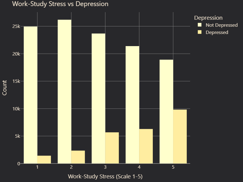

# Figure 9: Job-Study Satisfaction vs. Depression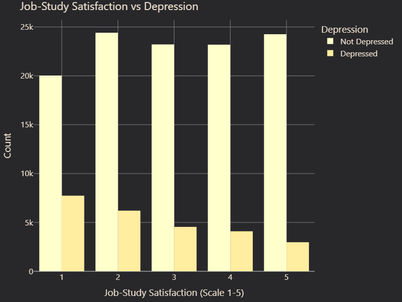

Reducing Dimensionality

Some features contained either erroneous values or a high number of unique values due to varied responses from surveyed individuals. This posed a problem because excessive feature uniqueness can lead to overfitting and reduced model interpretability. To address this, categorical variables such as Degree, Dietary Habits, and Sleep Duration were grouped into broader, more logical categories:

• Degree: Mapped into Secondary School, Undergraduate, Postgraduate, or Other.
• Dietary Habits: Categorized as Healthy, Moderate, Unhealthy, or Other (Figure 10).
• Sleep Duration: Grouped into Less than 5 hours, 5-6 hours, 7-8 hours, or More than 8 hours (Figure 11).

# Figure 10: Dietary Habits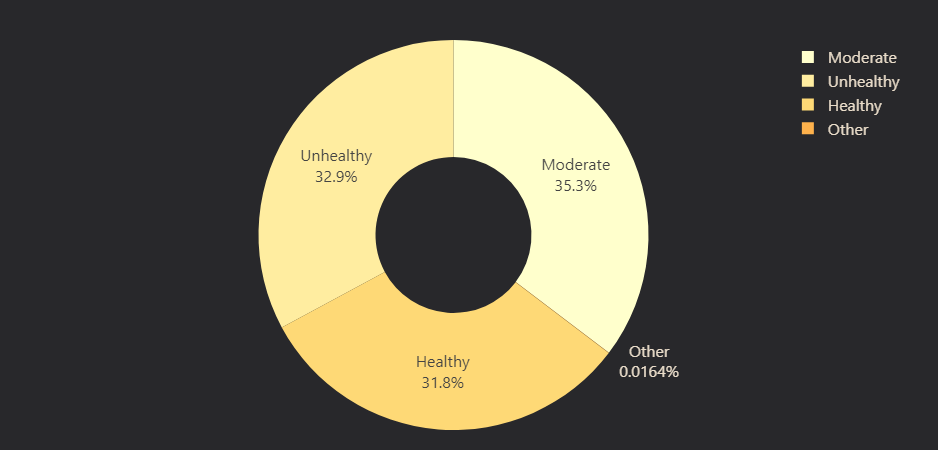

# Figure 11: Sleep Duration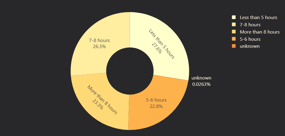

SHAP Analysis for Feature Importance

To refine the dataset further, we performed a SHAP (SHapley Additive exPlanations) analysis to understand the importance of each feature in predicting depression. SHAP values provide insights into how much each feature contributes to model predictions. The results indicated that City, Gender, and Family History of Mental Illness contributed very little to model performance (Figure 12). Since these variables did not significantly impact the predictions, they were removed from the feature pool.

# Figure 12: Feature Importance: SHAP analysis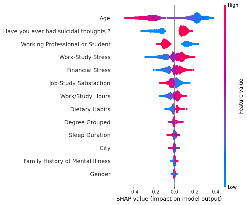

SHAP analysis serves as a critical step in feature selection, allowing us to retain only the most relevant features while discarding those that add little to no predictive power. This process not only improves model efficiency but also enhances interpretability by focusing on the factors that matter most in determining mental health outcomes.

By implementing these feature engineering strategies, we ensured that our dataset was not only cleaned of unnecessary noise but also structured in a way that maximized the predictive power of our model.

Machine learning model development is heavily reliant on the quality of data and its preprocessing. The models used in this study were designed to predict depression based on multiple psychological, demographic, and environmental factors. Given the imbalanced nature of the dataset, where non-depressed cases significantly outnumbered depressed cases, careful attention was given to balancing techniques and feature selection to enhance model performance.

Training and Model Selection

We employed the CatBoostClassifier, a gradient boosting algorithm that efficiently handles categorical features without extensive preprocessing. Two configurations were tested:

• Model 1: A CatBoostClassifier trained using default parameters.
• Model 2: A CatBoostClassifier with optimized hyperparameters.

Each model was trained on both imbalanced and balanced datasets. The balanced dataset was created through downsampling to equalize the number of cases in each class.

Performance Analysis

The impact of data balancing on model performance was evident in the results. Models trained on balanced data generalized significantly better for the minority class (depressed cases), regardless of whether they were tested on balanced or imbalanced datasets. In contrast, models trained on imbalanced data tended to favor the majority class, leading to lower recall for the depressed class.

A key observation was that while both the default and optimized models achieved comparable performance when trained on balanced data, the optimized model showed superior recall for the minority class when trained on the imbalanced dataset. This suggests that hyperparameter tuning can enhance learning for underrepresented labels in highly skewed datasets.

Key Classification Metrics

Below are key classification reports for selected models:

| Metric         | Class 0 | Class 1 | Macro Avg | Weighted Avg |
|----------------|---------|---------|-----------|--------------|
| Precision      | 0.84    | 0.97    | 0.90      | 0.90         |
| Recall         | 0.97    | 0.81    | 0.89      | 0.89         |
| F1-Score       | 0.90    | 0.88    | 0.89      | 0.89         |
| Accuracy       | 0.89    |         |           |              |
                

| Metric         | Class 0 | Class 1 | Macro Avg | Weighted Avg |
|----------------|---------|---------|-----------|--------------|
| Precision      | 0.93    | 0.91    | 0.92      | 0.92         |
| Recall         | 0.91    | 0.93    | 0.92      | 0.92         |
| F1-Score       | 0.92    | 0.92    | 0.92      | 0.92         |
| Accuracy       | 0.92    |         |           |              |
                

Key Findings

• Models trained on balanced datasets performed consistently better for Class 1 (depression), regardless of the test set used.
• There was no significant difference between the default and optimized models when trained on balanced data.
• When trained on imbalanced data, the optimized model outperformed the default model in classifying the minority class, with improved recall.
• Feature importance analysis highlighted work or study stress, suicidal thoughts, and academic pressure as the most influential factors in predicting depression.
• As expected, job and study satisfaction were negatively correlated with depression.
• Interestingly, dietary habits showed little correlation with depression based on this dataset.

Conclusions

Our findings emphasize the importance of handling data imbalance in mental health prediction models. The models trained on balanced datasets provided a more equitable distribution of recall and precision across both classes. Additionally, our results reinforce the need for robust exploratory data analysis, as key features such as occupational stress and suicidal thoughts played a dominant role in depression classification.

Future improvements may include exploring alternative modeling techniques, incorporating additional mental health indicators, and applying ensemble learning approaches to further enhance predictive power.

Walter Reade and Elizabeth Park. Exploring Mental Health Data. https://kaggle.com/competitions/playground-series-s4e11, 2024. Kaggle.